Tutorial

This tutorial shows some basic examples on how to import and use PyMaxflow. It is aimed to people who are already familiar with the maxflow problem and its applications in computer vision and image processing, and want to learn the basic usage of PyMaxflow. This is not, in any case, a tutorial on graph-cuts.

Getting started

Install PyMaxflow using pip:

pip install PyMaxflow

Once installed, import it as usual:

import maxflow

# Print the version
print(maxflow.__version__)

A flow network with two nodes

This example builds a simple flow network and finds its maximum flow.

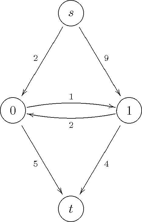
This network has two terminal nodes, the source and the sink , and two non-terminal nodes, labeled 0 and 1. In PyMaxflow, terminal nodes and are always implicitly present in the network, and it is not necessary (or even possible) to declare them explicitly. In addition, terminal edges (connecting non-terminal nodes with terminal nodes), and non-terminal edges (connecting non-terminal nodes), are treated differently.

The following code uses the standard single-edge methods of PyMaxflow to build this simple network. Note that these methods might be slow in practice for networks with many nodes and edges:

import maxflow

# Create a graph with integer capacities, with 2 non-terminal nodes and 2 non-terminal edges.
# Note that these numbers are just indicative (read below)
g = maxflow.Graph[int](2, 2)
# Add two (non-terminal) nodes. Get the index to the first one.
nodes = g.add_nodes(2)
# Create the non-terminal edges (forwards and backwards) with the given capacities between nodes 0 and 1.
g.add_edge(nodes[0], nodes[1], 1, 2)
# Set the capacities of the terminal edges...
# ...for the first node
g.add_tedge(nodes[0], 2, 5)
# ...for the second node
g.add_tedge(nodes[1], 9, 4)

The non-terminal edges are created with add_edge. The terminal edges are created with add_tedge.

The type of the capacities can be int, as in the example, or float. In that case, the graph declaration would be:

g = maxflow.Graph[float](2, 2)

The constructor parameters (2, 2) are initial estimations of the number of nodes and the number of non-terminal edges. These estimations do not need to be correct or even approximate (it is possible to set them to 0), but a good estimation allows for more efficient memory management. Consult the documentation of the constructor for more details. In this specific example, the number of nodes and non-terminal edges was known in advance.

Now we can find the maximum flow in the graph:

flow = g.maxflow()
print(f"Maximum flow: {flow}")

Finally, we want to know the the partition given by the minimum cut:

print(f"Segment of the node 0: {g.get_segment(nodes[0])}")
print(f"Segment of the node 1: {g.get_segment(nodes[1])}")

The method get_segment returns 0 when the given node belongs to the source partition and 1 when the node belongs to the sink partition.

This example is available in examples/simple.py. Running the code will print:

Maximum flow: 8
Segment of the node 0: 1
Segment of the node 1: 0

This means that the minimum cut cuts the graph in this way:

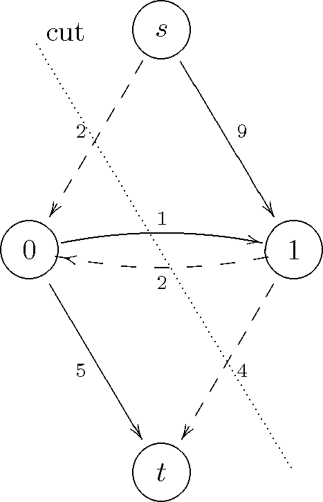
The severed edges are marked with dashed lines. Indeed, the sum of the capacities of these edges is equal to the maximum flow 8.

Binary image restoration

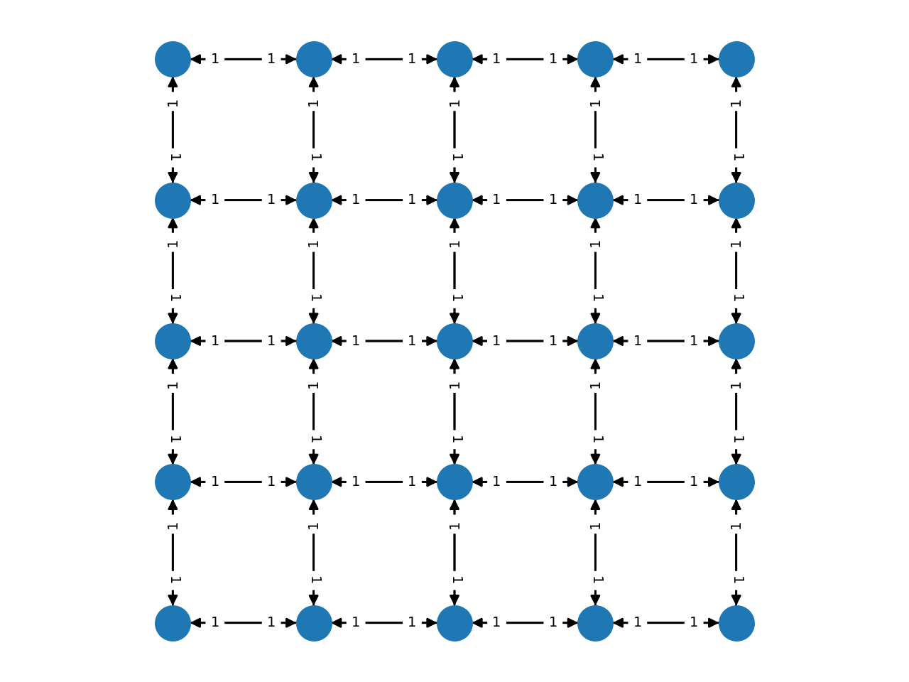
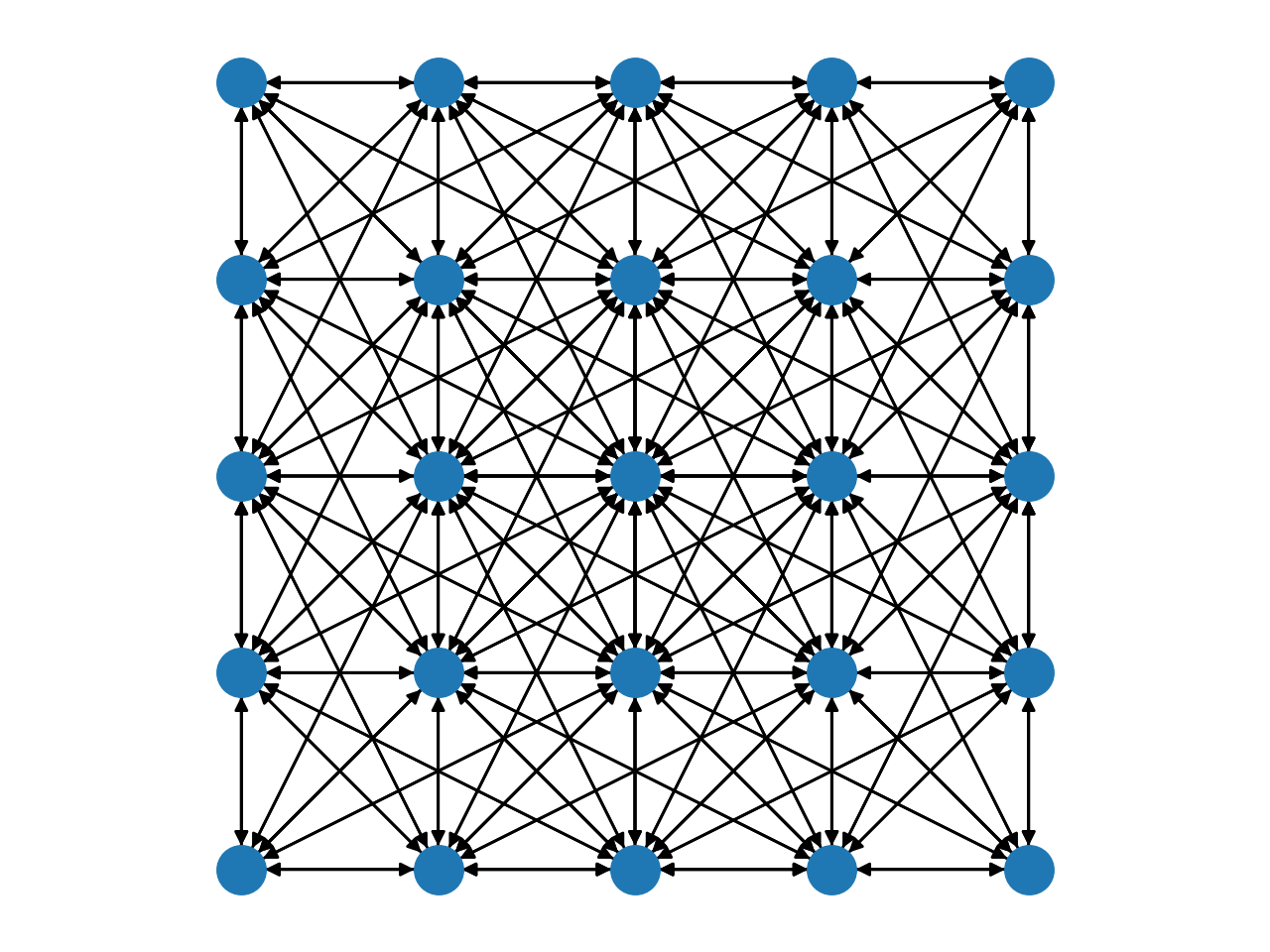
This example shows how to build a 4-connected grid layout of non-terminal nodes using the advanced multi-edge functions of PyMaxflow. While this example focuses on a relatively simple 4-connected grid, these multi-edge functions are flexible to create very complex networks involving many nodes and edges with a few calls. More details are given in the following section.

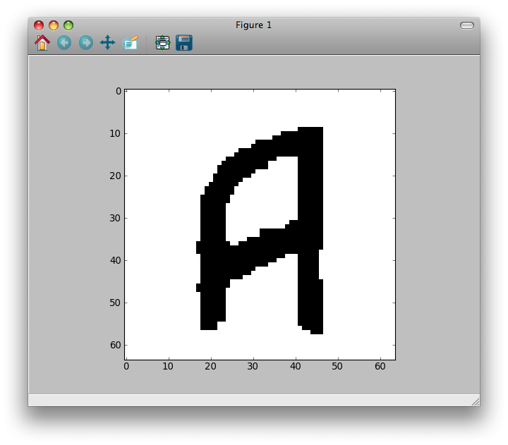
We will use the 4-connected grid network to remove Gaussian noise from a binary image. The original, noise-free image is

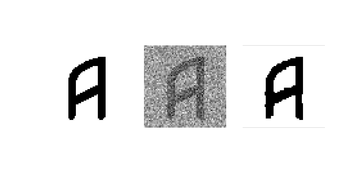
The noisy version was obtained adding strong Gaussian noise to the original image:

We will restore the image minimizing the energy

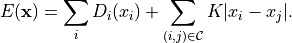
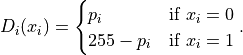
are the values of the restored image, is the number of pixels. The unary term (resp. ) is the penalty for assigning the value 0 (resp. 1) to the i-th pixel. Each depends on the values of the noisy image, which are denoted as :

Thus, is low when assigning the label 0 to dark pixels or the label 1 to bright pixels, and high otherwise. The value is the regularization strength. The larger the smoother the restoration. We arbitrarily fix it to 50.

The maximum flow algorithm is widely used to minimize energy functions of this type. We build a network to represent the above energy. This network has a non-terminal node per image pixel, and the nodes are connected in a 4-connected grid arrangement. The capacities of all non-terminal edges is . The capacities of the edges from the source node are set to , and the capacities of the edges to the sink node are .

Note

It could be possible to build this network as we did in the first example. First, add all the nodes with add_nodes. Then, iterate over the nodes adding the non-terminal edges with add_edge, and finally add the capacities of the terminal edges calling add_tedge once per pixel. While this approach is feasible, it is very slow in Python, especially when dealing with large images or stacks of images.

PyMaxflow provides methods for building complex networks with a few calls. The method add_grid_nodes adds multiple nodes and returns their indices in a convenient n-dimensional array with the given shape; add_grid_edges adds edges to the grid with a given neighborhood structure (4-connected by default); and add_grid_tedges sets the capacities of the terminal edges for multiple nodes:

# Create the graph.
g = maxflow.Graph[int]()
# Add the nodes. nodeids has the identifiers of the nodes in the grid.
# Note that nodeids.shape == img.shape
nodeids = g.add_grid_nodes(img.shape)
# Add non-terminal edges with the same capacity.
g.add_grid_edges(nodeids, 50)
# Add the terminal edges. The image pixels are the capacities
# of the edges from the source node. The inverted image pixels
# are the capacities of the edges to the sink node.
g.add_grid_tedges(nodeids, img, 255-img)

Perform the maxflow computation and get the results:

# Find the maximum flow.
g.maxflow()
# Get the segments of the nodes in the grid.
# sgm.shape == nodeids.shape
sgm = g.get_grid_segments(nodeids)

The method get_grid_segments returns an array with the same shape than nodeids. It is almost equivalent to calling get_segment once for each node in nodeids, but much faster, and preserving the shape of the input. For the i-th cell, the array stores False if the i-th node belongs to the source segment (i.e., the corresponding pixel has the label 1) and True if the node belongs to the sink segment (i.e., the corresponding pixel has the label 0). We now get the labels for each pixel:

# The labels should be 1 where sgm is False and 0 otherwise.
img2 = np.int_(np.logical_not(sgm))
# Show the result.
from matplotlib import pyplot as ppl
ppl.imshow(img2)
ppl.show()

The result is:

This is a comparison between the original image (left), the noisy one (center) and the restoration of this example (right):

Complex grids with add_grid_edges

The method add_grid_edges is a powerful tool to create complex network layouts:

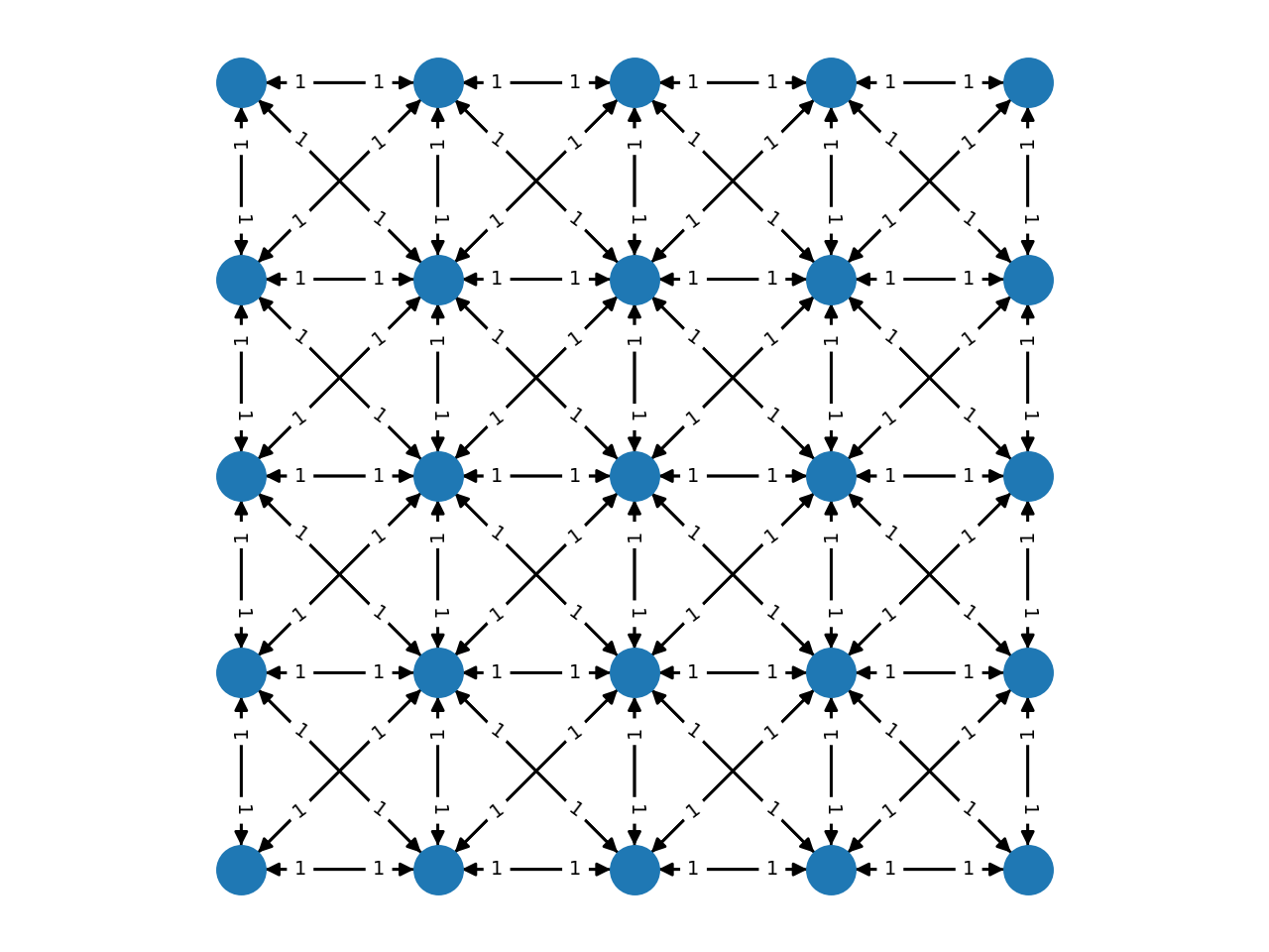
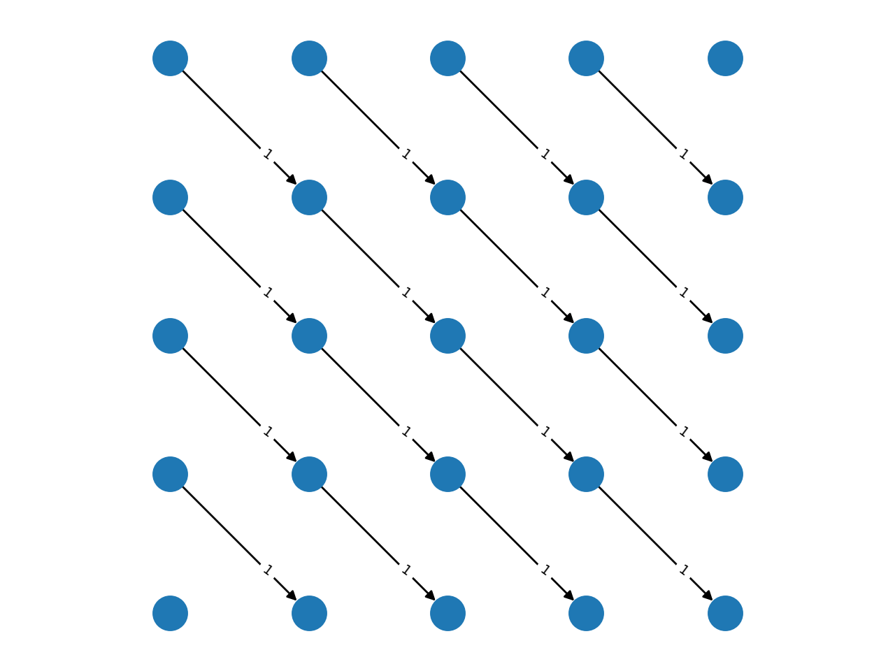
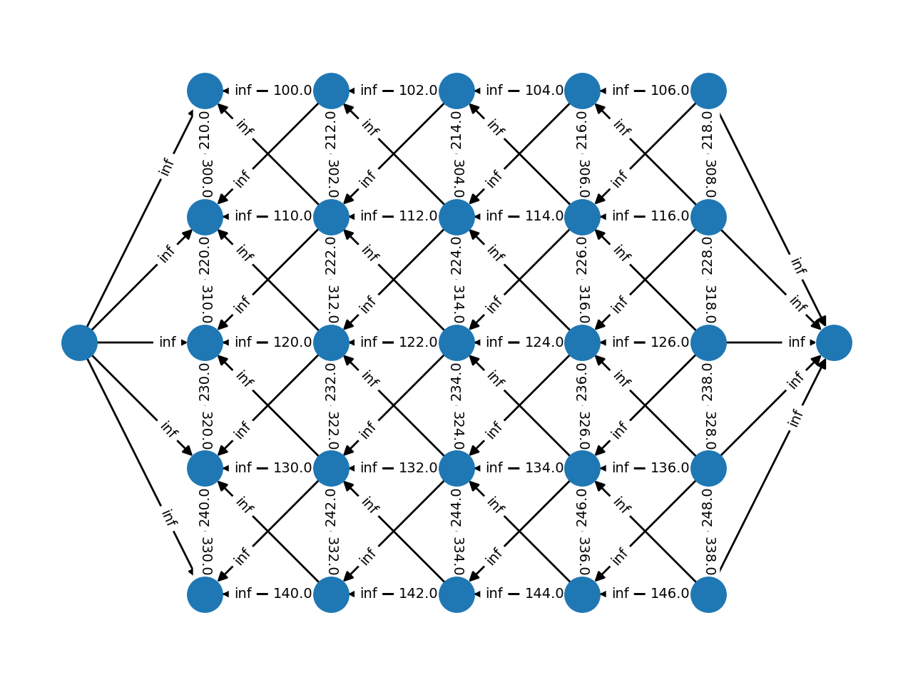
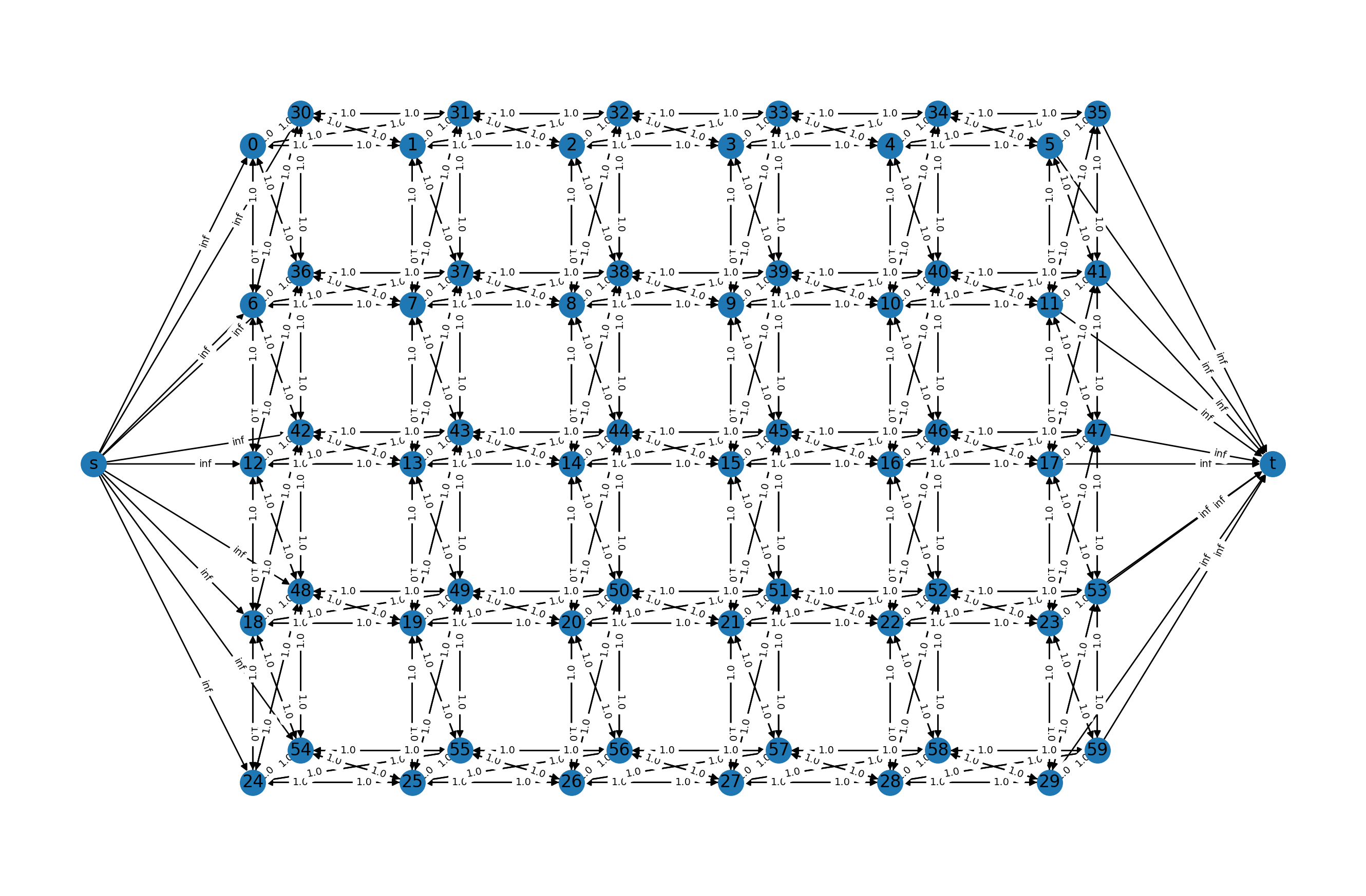
The best way to understand the potential applications of add_grid_edges is to look at the examples of the PyMaxflow repository.

• The file examples/layout_examples.py shows a variety of network layouts created with add_grid_edges.

• A more advanced example in examples/layout_example2.py builds a complex layout with several calls to add_grid_edges and add_grid_tedges.

• The file examples/layout_example3D.py contains the definition a 3D grid layout.

The documentation of maxflow.GraphInt.add_grid_edges() also contains a few useful use cases.